Amenity Detection and Beyond — New Frontiers of Computer Vision at Airbnb - 19 minutes read
 Amenity Detection and Beyond — New Frontiers of Computer Vision at Airbnb
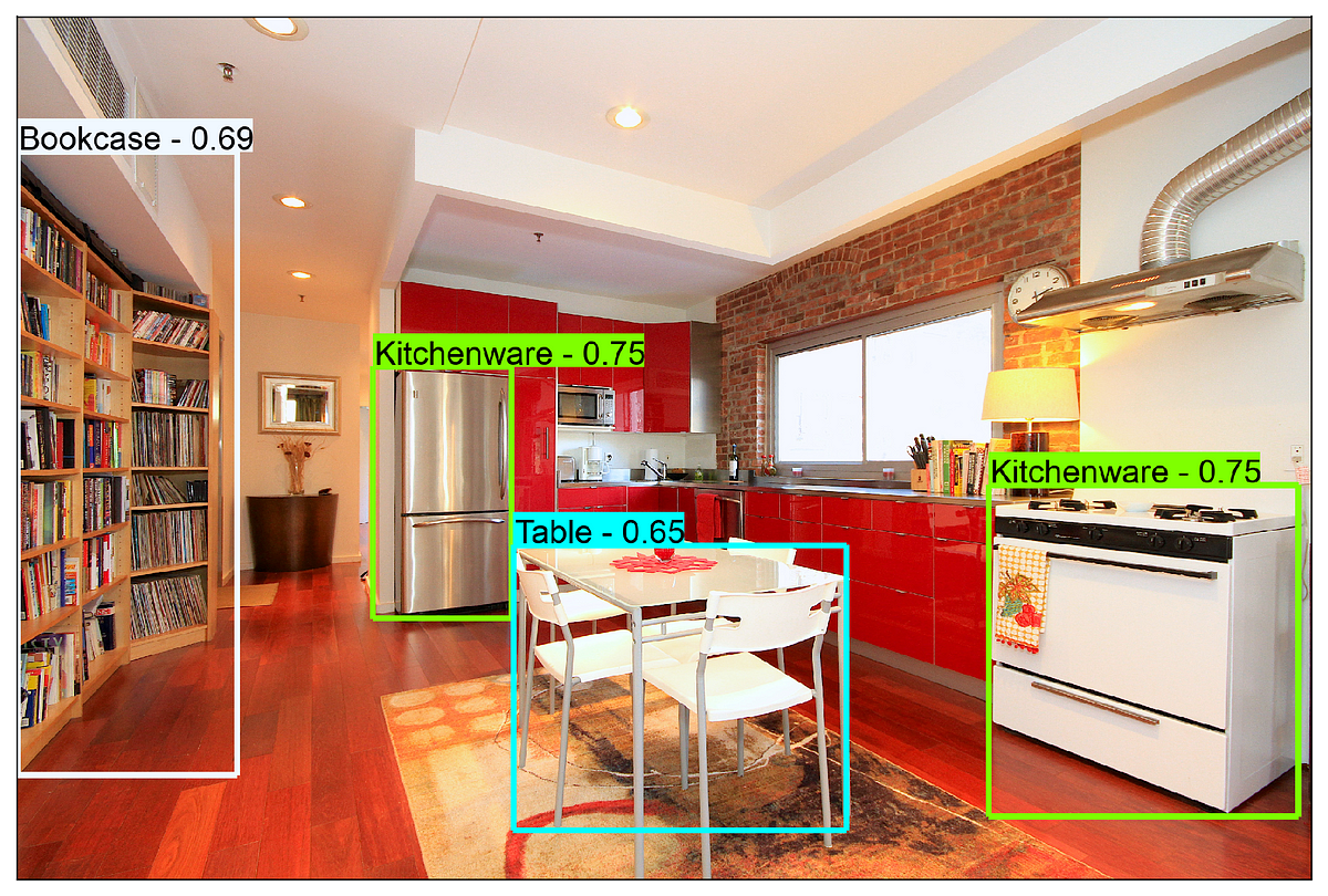
In 2018, we published a blog post titled Categorizing Listing Photos at Airbnb. In that post, we introduced an image classification model which categorized listing photos into different room types and helped organize hundreds of millions of listing photos on the Airbnb platform. Since then, the technology has been powering a wide range of internal content moderation tools, as well as some consumer-facing features on the Airbnb website. We hope such an image classification technology makes our business more efficient, and our products more pleasant to use. Image Classification is a sub-field of a broader technology called Computer Vision, which deals with how computer algorithms can be made to gain understandings of digital images or videos. Another related sub-field is Object Detection, which deals with detecting instances of semantic objects of a certain class in digital images or videos. Airbnb has millions of listings worldwide. To make sure our listings uphold high standards of quality, we need to determine whether the amenities advertised online match the actual ones. At our scale, using only human efforts to do so is obviously neither economical nor sustainable. Object Detection technologies, however, can lend us a helping hand, as amenities can be automatically detected in listing photos. Furthermore, the technology opens a new door to a home sharing platform where listing photos are searchable by amenities, which helps our guests navigate through listings much more easily. Object Detection technologies evolve rapidly. Just a few years ago, the idea to build an object detection model to detect amenities in a digital picture might sound prohibitively difficult and intimidating. Nowadays, a great number of decent solutions have already emerged, some of which require minimal efforts. For example, many third-party vendors provide generic object detection APIs which are usually quite cost-effective and easy to integrate into products. We tested a few different API services with our listing photos. Unfortunately, the results suggested that the APIs had quite noticeable gaps with our business requirement. The image below shows the results for a sample picture from our test data.
Even though the API service is able to detect certain amenities, the labels predicted are too vague. In a home sharing business like Airbnb, knowing that kitchenware exists in a picture does not tell us much other than the room type. Likewise, knowing there is a table in the picture doesn’t help us either. We don’t know what kind of a table it is, or what it could be used for. Our actual goal is to understand whether the detected amenities provide convenience for guests. Can guests cook in this home? Do they have specific cookware they want? Do they have a dining table of a decent size to host enough people if it is a family trip? A more desirable amenity detection result would look like something as below.
As one can see, the predicted labels are much more specific. We can use these results to verify the accuracy of listing descriptions and serve Homes searches to guests with specific amenity requests. In addition to the third-party API, open source projects like Tensorflow Detection Model Zoo and Detectron Model Zoo also offer a collection of free pre-trained object detection models, using different public image datasets and different model architectures. We tested various pre-trained models from the Model Zoos. Likewise, the results did not meet our requirement either. Precision was significantly lower and some predicted labels were just far off. These tests suggested that it was very much necessary for us to build a customized object detection model to solve our particular Amenity Detection problem. To do that, we needed to first determine what a customized set of amenities should be, build an image dataset based on that set of amenity labels, and have the images annotated with the labels. Through training against images with these annotations, we hope that the model can learn how to recognize these amenities, and then locate each instance detected. This is quite a long journey, and in the following sections, we will share how we walked through this whole process. Taxonomy is a scheme of amenity labels. Defining a taxonomy that encompasses amenities of our interest is a rather open-ended question. Ideally, the taxonomy should come from a specific business need. In our case, however, the taxonomy was unclear or varied from business units, so we bore the responsibility to come up with a minimal viable list first. This was quite a stretch as data scientists due to the limitations of our scope, but we believed that it could be a common problem to solve in many organizations. Our strategy was to get started with something lightweight, and then to iterate fast. Be an entrepreneur and never be shy to kick off the ball! Lacking prior experience, we decided to start from something people had worked on before, hopefully to find some hint. We found that Open Image Dataset V4 offered a vast amount of image data. It included about 9M images that had been annotated with image-level labels, object bounding boxes (BB), and visual relationships. In particular, BB annotations span a rich set of 600 object classes. These classes formed a hierarchical structure, and covered a wide spectrum of objects. On the highest level, they included Animal, Clothing, Vehicle, Food, Building, Equipment, Tool, and a collection of household items, such as Furniture, Appliances, and Home Supplies. Our goal was to find out the object classes that were relevant to amenities and to filter out the rest. We manually reviewed the 600 classes and selected around 40 classes that were relevant to our use case. They were generally important amenities in kitchen, bathroom, and bedroom, such as gas stove, oven, refrigerator, bathtub, shower, towel, bed, pillow,etc. Open Image Dataset V4 saved us a lot of time. If we were to start from scratch, building a reasonable taxonomy alone would have taken us a long time. After the taxonomy was determined, the next step would be to collect image data based on it. Open Image Dataset V4 had 14.6M BBs annotated in 1.7M images. Ideally, we could get a large number of image samples from it since our taxonomy was basically a subset of the complete 600 classes. However, as we dived deeper into the data, we found that the 600 object classes were highly imbalanced. Some classes had millions of instances while others only had a few.
The 40 classes of our interest mostly fell onto the minority (right) side of the class label distribution shown above. As a result, we ended up with only 100k instances of objects, annotated from about 50k images — about just 3% of the whole dataset. We had overestimated the amount of data available significantly! Modern object detection models are almost exclusively based on deep learning, which means they need a lot of training data to perform well. A general rule of thumb is that a few thousand image samples per class could lead to a decent model performance. 50k images annotated with 40 object classes implied 1.2k images per class on average, which was adequate, but not great. Therefore, we decided to add some in-house data, and to fuse it with the public data. To make sure the internal dataset includes rich, diverse, and evenly distributed amenity classes, we sampled 10k images for bedroom, bathroom, kitchen, and living room each, and additional 1k images for outdoor scenes such as swimming pool, view, and otherseach. Many vendors provide annotation services for object detection tasks. The basic workflow is that customers provide a labeling instruction and the raw data. The vendor annotates the data based on the labeling instruction and returns the annotations. A good labeling instruction makes the process move smoothly and yields high-quality annotations, and is therefore extremely important. Try to be as specific as you can, and always provide concrete examples. Writing a thoughtful one all at once is usually impossible, especially if you are doing this for the first time, so be prepared to iterate. In this project we chose Google data labeling service which three things we really liked about: 1) supporting up to 100 object classes for labeling, 2) a nice and clean UI where we could monitor the progress of the labeling job, and 3) feedback and questions were constantly sent to us as the labeling work moved forward. As a result, we were able to make vague instructions clear and address edge cases in the whole process. One important strategy was to send small batches of data before ramping up. In that way, you get the opportunity to correct your labeling instruction and have the majority of your data annotated with an improved version. In our experience, we found some amenities were ubiquitous and less useful (e.g. curtains, windows) in these small-batch results. We took them out accordingly and refined our taxonomy from 40 classes down to 30. Afterward we had our data completely annotated in about two weeks.
Combining the labeled 43k internal images and the 32k public images, we ended up with 75k images annotated with 30 customized amenity objects. Now it was time to actually build the model! We tried two paths building the model. One path was to leverage the Tensorflow Object Detection API — creating tfrecords based on the annotated image data, using the model_main.py to kick off the training, and running Tensorboard to monitor the training progress. There were many online tutorials on how to do that. We will skip most details here and only cite our favorite one. In particular, we chose two pre-trained models for fine tuning: ssd_mobilenet_v2and faster_rcnn_inception_resnet_v2. ssd_mobilenet_v2 was fast, but with lower accuracy, and faster_rcnn_inception_resnet_v2 was the opposite. To set up a benchmark, we tested the accuracy of both pre-trained models on a 10% held-out data (7.5k images with 30 object classes) before fine tuning. We use mean Average Precision (mAP) as the metric, which is standard for evaluating an object detection model. It measures the average precision (AUC of a precision-recall curve) of a model across all object classes, and ranges between 0 and 1. More details are explained here. ssd_mobilenet_v2 achieved mAP of 14% and faster_rcnn_inception_resnet_v2 achieved mAP of 27%. A careful reader may find that our benchmark results for these two pre-trained models were much lower than the reported mAPs on the website: 36% for ssd_mobilenet_v2, and 54% for faster_rcnn_inception_resnet_v2. This was not incorrect. Our test set had only 30 classes, all of which were minority ones in the dataset where the pre-trained model was trained. The degradation of accuracy for the pre-trained models was due to a shift in class distribution between training and test sets. To start training on our dataset, we froze parameters in feature extraction layers, and only made the fully connected layers trainable. The default initial learning rate was 8e-4 for ssd_mobilenet_v2 and 6e-5 for faster_rcnn_inception_resnet_v2. Since we were doing transfer learning, we lowered the learning rates to only 10% of the default values. The rationale was that we did not want to make too large of a gradient update to “destroy” what had already been learned in the pre-trained model weights. We also decreased the number of training steps from 10M to 1M and scaled corresponding decay parameters in the learning rate schedule. In terms of computing resource, an AWS p2.xlarge instance, with Tesla K80 single-core GPU was used for the training job. When training ssd_mobilenet_v2, the loss function decreased very fast in the beginning. However, after 100k steps (5 days), the improvement became marginal, and the loss function began to oscillate. Unsure if continuing the training would still make sense, we stopped the training after 5 days because the progress was anyways too slow. The model accuracy (mAP) increased from 14% to 20%. When training faster_rcnn_inception_resnet_v2, the loss function started very small, but immediately began to show lots of wild behavior. We were not able to improve the mAP of the model at all. We estimated that an mAP of at least 50% was needed to build a minimal viable product, and there was obviously still a big gap. By this point we had spent a lot of time dealing with model training. We hypothesized that the loss function probably got stuck at some local minima, and we needed to apply some numerical tricks to jump out of it. The diagnosis would be quite involved. Meanwhile, switching to other model architecture which was easier to retrain was definitely an option too. We decided to leave off there, and planned to revisit the problem in the future. Another path to build the model was through an automated self-service tool. We tried Google AutoML Vision. Surprisingly, the results were very impressive. Just by uploading the 75k annotated images and clicking a few buttons, we were able to train an object detection model in 3 days. We opted in higher accuracy in the self-service menu so the training took longer than usual. We chose to use the model trained by AutoML. The model achieved an mAP of about 68% based on our offline evaluation in a 10% held-out data (7.5k images). The result is significantly higher than all the metrics we had seen so far. Certain classes had particularly great performance, such as Toilet, Swimming pool,andBed, all achieving 90%+ average precision. The worst performing classes were Porch, Wine rack,and Jacuzzi. We found that the average precision of each object class was strongly correlated with its prevalence in the training data. Therefore, increasing training samples for these minority classes would likely improve the performance of those categories a lot.
In our offline evaluation, we also found that mAP was quite sensitive to training-test split. A different split due to simple statistical randomness could lead to 2–3% drift. The major instability of mAP came from minority classes where the sample size was very small. We recommend using the median of APs of all classes to mitigate this problem. Model deployment on AutoML was also extremely easy, with only one click. After deployment, the model was turned into an online service which people could easily use through REST API or a few lines of Python code. Queries-per-Second (QPS) can vary depending on the number of node hours deployed. A big downside of AutoML though was that you could not download the original model you created. This was a potential problem and we decided to revisit it in the future. Finally, we want to demonstrate the performance of our model by showing a few more concrete examples, where our customized model will be compared against an industry-leading third-party API service. Please note that our taxonomy only includes 30 amenity classes, but the API service includes hundreds.
As one can see, our model is considerably more specific and provides much wider coverage for these 30 object classes. A more quantitative comparison between our model and the third-party model in this demo needs some careful thoughts. First, our taxonomy is different from that of the third-party model. When calculating mAP, we should include only the intersection of the two class sets. Second, the third-party API only shows partial results as any predictions with a confident score less than 0.5 would have been filtered and not observable by us. This basically truncates the right side of the precision-recall curve of their results where recall is high (and threshold is low), and thus lowers the mAP of their results. To make a fair comparison, we should truncate our results by removing detections whose scores are less than 0.5 too. After the treatment, we calculated that the “truncated” mAP for our model was 46%, and 18% for theirs. It is really encouraging to see that our model can significantly outperform a third-party model from an industry-leading vendor. The comparison also demonstrates how important domain-specific data is in the world of computer vision.
In addition to Amenity Detection, Object Detection with broader scope is another important area that we are investing in. For example, Airbnb leverages many third-party online platforms to advertise listings. To provide legitimate ads, we need to make sure the displayed listing photos do not pose excessive privacy or safety risks for our community. Using Broad-scope Object Detection, we are able to perform necessary content moderation to prevent things like weapons, large-size human faces, etc. from being exposed without protection. We are currently using Google’s Vision service to power this. We are also building a configurable detection system called Telescope, which can take actions on images with additional risky objects when necessary. Another growing need in our business is to use AI to assist our process of quality control for listing images. As an early adopter, we leveraged a new technology that Google is working on, and designed a better set of catalog selection criteria for both re-marketing and prospecting campaigns. The technology supports two models: One predicts an aesthetic score, and the other predicts a technical score. The aesthetic score evaluates the aesthetic appeal of the content, color, picturing angle, sociality, etc., while the technical score evaluates noise, blurriness, exposure, color correctness, etc. In practice, they complement each other very well. For example, the image below was once in our advertisement catalog. Now that we understand that it has a high technical score but a poor aesthetic score, we can comfortably replace it with a more attractive yet still informative image.
Source: Medium.com
Powered by NewsAPI.org
Keywords:
Computer vision • Airbnb • Blog • Photograph • Airbnb • Computer vision • Scientific modelling • Airbnb • Technology • Internet forum • Tool • Consumer • Airbnb • Website • Computer vision • Technology • Business • Efficiency • Product (business) • Computer vision • Discipline (academia) • Technology • Computer vision • Algorithm • Digital image • Object detection • Semantics • Airbnb • Sustainable design • Technology • Technology • Technology • Scientific modelling • Application programming interface • Product (business) • Application programming interface • Application programming interface • Requirement • Image • Image • Application programming interface • Airbnb • Application programming interface • Open-source model • TensorFlow • Zoo (file format) • Free software • Conceptual model • Conceptual model • Conceptual model • Accuracy and precision • Prediction • Test (assessment) • Conceptual model • Problem solving • Image • Data set • Image • Annotation • Scientific modelling • Open-ended question • Environmental economics • Organization • Entrepreneurship • Image • Image • Data • Image • Image • Hierarchy • Clothing • Vehicle • Food • Building • Machine • Tool • Furniture • Home appliance • Home • Goal • Use case • Kitchen • Bathroom • Bedroom • Gas stove • Oven • Refrigerator • Bathtub • Shower • Towel • Bed • Pillow • Scratch building • Time • Image • Data • Open-source software • Image • Data set • Bulletin board system • Image • Number • Image • Subset • Data • Object (computer science) • Class (computer programming) • Class (computer programming) • Instance (computer science) • Class (computer programming) • Class (computer programming) • Object (computer science) • Object (computer science) • Data set • Object detection • Mathematical model • Deep learning • Rule of thumb • Image • Class (computer programming) • Mathematical model • Object-oriented programming • Bedroom • Bathroom • Kitchen • Living room • Swimming pool • Service (economics) • Workflow • Customer • Packaging and labeling • Return on investment • Scientific method • Google • Data • Object-oriented programming • Clean technology • User interface • Feedback • Data • TensorFlow • Application programming interface • Digital image • Data • Scientific modelling • Python (programming language) • Solid-state drive • ResNet • Solid-state drive • ResNet • Specification (technical standard) • Data • Class (computer programming) • Information retrieval • Function (mathematics) • Metric (mathematics) • Statistical model • Information retrieval • Integral • Precision and recall • Conceptual model • Solid-state drive • ResNet • Specification (technical standard) • Map • Solid-state drive • ResNet • Data set • Mathematical model • Accuracy and precision • Conceptual model • Social class • Probability distribution • Statistical hypothesis testing • Training • Data set • Parameter • Feature extraction • Solid-state drive • ResNet • Inductive transfer • Slope • Rate schedule (federal income tax) • System resource • Amazon Web Services • X-Large • Tesla (microarchitecture) • Graphics processing unit • Solid-state drive • Loss function • Loss function • ResNet • Loss function • Scientific modelling • Environmental economics • Time • Scientific modelling • Loss function • Maxima and minima • Numerical analysis • Bayesian network • Scientific modelling • Architecture • Problem solving • Automation • Tool • Google • Computer vision • Object detection • Conceptual model • Map • Evaluation • Swimming pool • Information retrieval • Wine rack • Jacuzzi • Information retrieval • Sample (statistics) • Social class • Evaluation • Statistical hypothesis testing • Statistical randomness • Function (mathematics) • Sample size determination • Median • Statistical model • Representational state transfer • Python (programming language) • Queries per second • Queries per second • Number • Mathematical model • Industry • Application programming interface • Service (economics) • Taxonomy (general) • Application programming interface • Conceptual model • Technology demonstration • Thought • Taxonomy (general) • Conceptual model • Function (mathematics) • Intersection (set theory) • Class (set theory) • Set (mathematics) • Application programming interface • Prediction • Observation • Precision and recall • Scientific modelling • Domain-specific language • Data • Computer vision • Airbnb • Advertising • Advertising • Privacy • Security • Google • Power (social and political) • System • Telescope • Image • Risk • Business • Artificial intelligence • Scientific method • Quality control • Image • Early adopter • Technology • Google • Marketing • Marketing • Technology • Conceptual model • Aesthetics • Technology • Aesthetics • Aesthetics • Color • Color • Complementary colors • Image • Advertising • Aesthetics • Information • Image •